> For the complete documentation index, see [llms.txt](https://notes.dizy.cc/llms.txt). Markdown versions of documentation pages are available by appending `.md` to page URLs; this page is available as [Markdown](https://notes.dizy.cc/fundamental-algorithms/search-trees.md).
# Search Trees
## Binary Search Trees (BST)
{% hint style="info" %}
Related homework questions: h3-6
{% endhint %}
### Binary Tree
A binary tree $$T$$ is a set $$N$$ of nodes where each node $$u\_0$$ has two pointers, $$u\_0$$.left and $$u\_0$$.right.
The size of $$T$$ is $$|N|$$.
**Complete Binary Tree**
Every level of the tree is completely filled, except possibly the last level. Moreover, the last level has to be filled from left to right.
If a complete binary tree is also complete on the last level, then it is called a **perfect** binary tree.
**Height of binary trees**
Minimum number of nodes in a binary tree of height $$h$$:
$$
\begin{gather\*} \mu(h) = h + 1 \end{gather\*}
$$
Maximum number of nodes in a binary tree of height $$h$$:
$$
\begin{gather\*} M(h) = 2^{h+1} - 1 \end{gather\*}
$$
The minimum height of binary trees with $$n$$ nodes:
$$
\begin{gather\*} h \ge \lg(n + 1) - 1 \end{gather\*}
$$
### Binary Search Tree
A binary tree is a binary search tree if each node $$u \in T$$ has a field $$u$$.key that satisfies the BST property:
$$
\begin{gather\*} u\_L.key < u.key \le u\_R.key \end{gather\*}
$$
## AVL Trees
{% hint style="info" %}
Related homework questions: h3-7, h3-8
{% endhint %}
An AVL tree is a binary search tree where the left subtree and right subtree at each node differ by at most 1 in height.
### Balance Factor
More generally, define the **balance** of any node $$u$$ of a binary tree to be the height of the left subtree minus the height of the right subtree:
$$
\begin{gather\*} b(u) = h(u.left) - h(u.right) \end{gather\*}
$$
### Insertion and Deletion Algorithms
**UPDATE PHASE**: Insert or delete as we would in a binary search tree.
**REBALANCE PHASE**: Let $$x$$ be parent of the node that was just inserted, or just cut during deletion, in the UPDATE PHASE. THe path from $$x$$ to the root will be called the **rebalance path**. We now move up this path, rebalancing nodes along this path as necessary.
Let $$u$$ be the first unbalanced node we encounter along the rebalance path from bottom to top. It is clear that $$u$$ has a balance of $$\pm 2$$. The situation is illustrated below:

#### Insertion Rebalancing
CASE (I.a): $$h\_L = h$$ and $$h\_R = h - 1$$. This means that the inserted node is in the left subtree of $$v$$. In this case, we rotate $$v$$, the result would be balanced. Moreover, the height of $$u$$ is now $$h+1$$. We call this the "single-rotation" case.

CASE (I.b): $$h\_L = h - 1$$ and $$h\_R = h$$. This means that the inserted node is in the right subtree of $$v$$. In this case, let us expand the subtree $$D$$ and let $$w$$ be its root. The two children of $$w$$ will have heights $$h - \delta$$ and $$h - \delta'$$ where $$\delta, \delta' \in {1, 2}$$. Now a double-rotation at $$w$$ results in a balanced tree of height $$h+1$$ rooted at $$w$$.

#### Deletion Rebalancing
CASE (D.a): $$h\_L = h$$ and $$h\_R = h - 1$$. This is like case (I.a) and treated in the same way, namely a single rotation at $$v$$. Now $$u$$ is replaced by $$v$$ after this rotation, and the new height of $$v$$ is $$h+1$$. Now $$u$$ is AVL balanced. However, since the original height is $$h + 2$$, there may beb unbalanced node further up the rebalance path. Thus, this is a non-terminal case.
CASE (D.b): $$h\_L = h - 1$$ and $$h\_R = h$$. This is like case (I.b) and treated in the same way, namely a double rotation at $$w$$. Again, this is a non-terminal case.
CASE (D.c): $$h\_L = h\_R = h$$. This case is new, we simply rotate at $$v$$. We check that $$v$$ is balanced and has height $$h+2$$. Since $$v$$ is in the place of $$u$$ which has height $$h+2$$ originally, we can safely terminate the rebalancing process.

## Ratio/Weight Balanced Trees
{% hint style="info" %}
Related homework questions: h4-3
{% endhint %}
**Extended size**:
$$
\begin{gather\*} esize(u) = \begin{cases} 1 & \text{if } u = nil \ esize(u.left) + esize(u.right) & \text{if } u \neq nil \end{cases} \end{gather\*}
$$
**Ratio**:
$$
\begin{gather\*} ratio(u) := {esize(u.left) \over {esize(u.right)}} \end{gather\*}
$$
### ρ-ratio
$$
\begin{gather\*} \rho < ratio(u) < 1/\rho \end{gather\*}
$$
### Insertion and Deletion Algorithms
Example: $$ho = 1/3$$
**UPDATE PHASE**: Insert or delete as we would in a binary search tree. In insertion, this results in a new leaf $$x$$ in $$T$$. If deletion, we will physically "cut" the leaf $$x$$ from $$T$$.
**REBALANCE PHASE**: Let $$u$$ be the parent of $$x$$. Clearly, every node that is not RB balanced must lie on the root-path of $$u$$. We therefore move up this path, rebalancing any such node.
```
Rebalance(u)
While (u != u.parent)
u <- Rebalance-Step(u)
u <- u.parent
```
```
Rebalance-Step(u)
If (ratio(u) >= 3)
v <- u.left
If (ratio(v) >= 3/5)
Return(rotate(v))
Else \\ ratio(v) < 3/5
Return(double-rotate(v.right))
elif (ratio(u) <= 1/3)
v <- u.right
If (ratio(v) <= 3/5)
Return(rotate(v))
Else \\ ratio(v) > 3/5
Return(double-rotate(v.left))
else
Return(u)
```
## Generalized B-Trees: (2,3)-trees
{% hint style="info" %}
Related homework questions: h4-1, h4-2
{% endhint %}
An (a,b)-tree is a rooted, ordered tree with the following structural constraints:
* Depth property: All leaves are at the same depth.
* Degree bound: Let $$m$$ be the number of children of an internal node $$u$$. This is also known as the **degree** of $$u$$. In general, we have the bounds $$a \le m \le b$$.
The root is an exception, with the bound $$2 \le m \le b$$.
### (a,b)-search trees
> Lecture Note 3, Page 80.
An (a,b)-search tree is an (a,b)-tree whose nodes are organized as an **external search tree**, which means items are only stored in leaves. Leaves are also called **external nodes**.

Leaves: $$(a', b')$$ where $$1 \le a' \le b'$$.
Default assumption for leaves: $$a' = b' = 1$$.
#### Reorganization of nodes
For an internal node $$u$$,
* $$u$$ is **overfull** if its degree is $$b+1$$.
* $$u$$ is **underfull** if its degree is $$a-1$$.
**Simple Remedy**: borrow or donate children

**Strong Remedy**: when simple remedy fails.
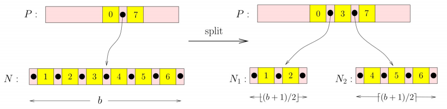
* Split an overfull node
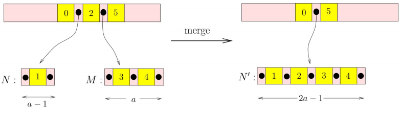
 * Merge an underfull node
 #### Split-Merge Inequality
$$
\begin{gather\*} a \le {{b + 1} \over {2}} \end{gather\*}
$$
This is a combination of split inequality ($$a \le \lfloor{{b+1}\over{2}}\rfloor$$) and merge inequality ($$a \le {{b + 1} \over {2}}$$). Since $$a$$ and $$b$$ are integers, these two are equivalent.
#### Split-Merge Inequality
$$
\begin{gather\*} a \le {{b + 1} \over {2}} \end{gather\*}
$$
This is a combination of split inequality ($$a \le \lfloor{{b+1}\over{2}}\rfloor$$) and merge inequality ($$a \le {{b + 1} \over {2}}$$). Since $$a$$ and $$b$$ are integers, these two are equivalent.